Method overview
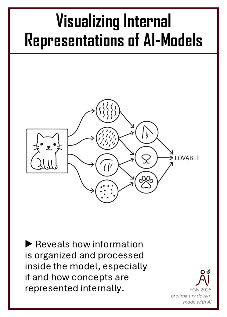
Goals: Visualize model-internal representations to better understand the black-box behavior and get an idea of whether the model has learned plausible representations/features from the data.
What it does: t-SNE takes messy, high-dimensional data and produces a two-dimensional map where “things” that are alike stay together. Its goal is to preserve neighborhoods, not exact distances.
Limitations: t-SNE is primarily used for visualization, rather than precise measurement. Distances inside a cluster are meaningful, but distances between clusters are not always reliable.
XAI taxonomy: model-agnostic, post-hoc, global
Details and further intuition
Step 1. We start with data points \( x_1, \ldots, x_n \) in high-dimensional space.
We want to measure the similarity between each pair. t-SNE does this by turning distances into conditional probabilities:
\[p_{j | i} = \frac{\exp(-\|x_i-x_j\|^2 / 2\sigma_i^2)}{\sum_{k\neq i}\exp(-\|x_i-x_k\|^2 / 2\sigma_i^2)}\]
Intuitively, this is like asking “How likely is \( x_j \) to be a neighbor of \( x_i \).” Here, \(\sigma_i\) is a parameter that controls how spread out the density is. The conditional probability is not symmetric, so t-SNE then sets
\[ p_{ij} = \frac{p_{j | i} + p_{i | j}}{2n},\quad p_{ii}=0, \qquad i,j=1,\ldots,n. \]
This gives a probability distribution over all pairs because \( \sum_{i, j} p_{ij} = 1\). The benefit of this distribution is that it reflects high-dimensional neighborhoods.
Step 2. Now, t-SNE needs to find a low-dimensional “embedding”, that is, corresponding points \(y_1, \ldots, y_n\).
We want a similar neighborhood structure. For this, we also need a neighborhood measure for the points in the low-dimensional space. There exist several versions to do it. All of them center around the idea of using a heavy-tailed Student-t distribution to avoid overly crowded points. Here, we use
\[q_{ij} = \frac{\exp(-\|y_i-y_j\|^2)}{\sum_{k\neq l}\exp(-\|y_k-y_l\|^2)}.\]
Nearby points have high \( q_{ij} \), but distant points still get some small probability thanks to the heavy tail.
Step 3. We still need to determine the low-dimensional points \(y_1, \ldots, y_n\). For this, we want the low-dimensional similarities \(q_{ij}\) to match the high-dimensional similarities \(p_{ij}\). t-SNE achieves this by minimizing the KL divergence
\[ C = KL( P \| Q) = \sum_{i\neq j} p_{ij} \log\frac{p_{ij}}{q_{ij}}, \]
where \(P\) and \(Q\) denote the neighborhood probability distributions in both the high- and the low-dimensional space. This cost \(C\) is asymmetric: it heavily penalizes if a high-dimensional neighbor (\(p_{ij}\) large) ends up far away in low-dim space (\(q_{ij}\) small). But if two points are far apart in high-dimensional space, we don’t care much if they get closer in low-dimensional space (as long as they don’t become too crowded).
Step 4. The last step is to optimize the cost function \(C\) from step 3. This is achieved using gradient-descent-type algorithms, which involve adjusting the positions of the low-dimensional points \(y_1, \ldots, y_n\).
The gradient has the form
\[ \frac{\partial C}{\partial y_i} = 4 \sum_j (p_{ij}-q_{ij})(y_i-y_j)(1+\|y_i-y_j\|^2)^{-1}. \]
This pushs \(y_{i}\) and \(y_{j}\) closer if \(p_{ij}> q_{ij}\). Conversely, this pushs \(y_{i}\) and \(y_{j}\) apart if \(p_{ij}< q_{ij}\). The Student-t tail ensures distant points don’t all collapse into the center.
Some words about the algorithm parameters:
- perplexity: more or less a target number of neighbors. For a low number, t-SNE only considers “close” neighbors; for higher numbers, more distant neighbors can also be taken into account.
- Learning rate: t-SNE internally runs an optimization problem; the learning rate controls how fast the positions of the 2D-projected points change (users can usually stick with the default value).
Further resources
- original paper: Visualizing Data using t-SNE (more than 60k citations)
- t-SNE clearly explained. An intuitive explanation of t-SNE | Medium
- other visualization methods: PCA (very basic dimension reduction), UMAP
- Code/Packages/Implementations: